
Overview
I recently had the pleasure of delving into the workings of a novel deep learning-based SLAM system, which I studied for my Advanced Machine Learning course project presentation at Northeastern University. Here I am going to discuss workings of SLAM system and go through important concepts of visual slam from other papers that will make understanding of this paper easier. If you have any questions, I’d be more than happy to assist you.
Visual SLAM
Visual SLAM is an algorithm that takes monocular, stereo, or RGB-D images as input and produces a dense or sparse depth map along with a camera trajectory. A key element for accuracy has been full Bundle Adjustment (BA), which jointly optimizes the camera poses and the 3D map in a single optimization problem. Despite significant progress, current SLAM systems lack the robustness demanded for many real-world applications. Failures can occur in many forms, such as lost feature tracks, divergence in the optimization algorithm, and accumulation of drift. Zachary Teed and Jia Deng from Princeton University addressed these problems by introducing a new deep learning-based solution to the SLAM system.
Optical Flow
In order to understand how droidslam works, it is important to first grasp the concept of Optical Flow, which is a fundamental topic in computer vision. Optical flow is the task of estimating per-pixel motion between video frames.


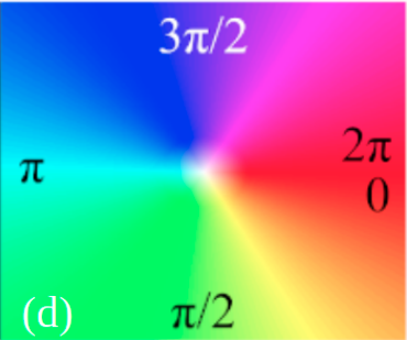 Dense Color Mapped Optical Flow
It results in a 2D vector field where each vector represents the displacement of points from one frame to the next. These vectors are then color-coded to represent their direction and intensity, resulting in a dense color output. Optical flow relies on certain assumptions, such as the idea that object pixel intensities remain constant between consecutive frames and that neighboring pixels exhibit similar motion.
Application of Optical Flow
In the ball game, I use the RAFT algorithm to calculate the optical flow between successive frames. Ball is then moved in direction of the optical flow which is taken at center of current ball position. I also apply a gravity vector to the ball’s trajectory at every frame to simulate the effect of gravity.
RAFT1 extracts perpixel features, builds multi-scale 4D correlation volumes for all pairs of pixels, and iteratively updates a flow field through a recurrent unit that performs lookups on the correlation volumes. Current DROID-SLAM is heavily inspried from the RAFT algorithm.
DROID SLAM2
DROIDSLAM is a visual slam that consists of recurrent iterative updates of camera pose and pixelwise depth through a Dense Bundle Adjustment layer. Despite training on monocular video, it can leverage stereo or RGB-D video to achieve improved performance at test time. DROID-SLAM is accurate, achieving large improvements over prior work, and robust, suffering from substantially fewer catastrophic failures.
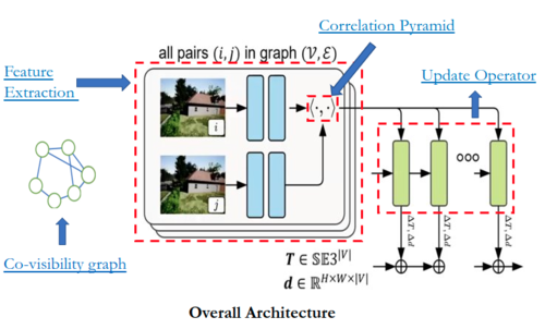
 DROID SLAM OVERVIEW
The strong performance and generalization of DROID-SLAM is made possible by its “Differentiable Recurrent Optimization-Inspired Design” (DROID), which is an end-to-end differentiable architecture that combines the strengths of both classical approaches and deep networks. Specifically, it consists of recurrent iterative updates, building upon RAFT for optical flow but introducing two key innovations. First, unlike RAFT, which iteratively updates optical flow, we iteratively update camera poses and depth. Second, each update of camera poses and depth maps in DROID-SLAM is produced by a differentiable Dense Bundle Adjustment (DBA) layer.
Architecture
click the image hyperlinks to learn more about each module
Network operates on an ordered collection of images, \({I_t}_{t=0}^{N}\). For each image $t$ has two state variables camera pose \(G_t \in SE(3)\) and inverse depth \(d_t \in \mathbb{R}^{H \times W}{+}\) . The set of poses, \({G_t}_{t=0}^{N}\), and set of inverse depths \({d_t}_{t=0}^{N}\) are unknown state variables, which get iteratively updated during inference as new frames are processed. Depth here refer to inverse depth parameterization.
Co-visibility Graph
Frame-graph $(V, E)$ to represent co-visibility between frames. An edge $(i , j) ∈ E $ means image $I_i$ and $I_j$ have overlapping fields of view which shared points. The frame graph is built dynamically during training and inference. After each pose or depth update, we can recompute visibility to update the frame graph. If the camera returns to a previously mapped region, add long range connections in the graph to perform loop closure.
 Frame Graph during SLAM initialization with 12 images
Feature Extraction
DROID has two separate networks, a feature network and context network. Each network consists of 6 residual blocks and 3 downsampling layers, producing dense feature maps at $1/8$ the input image resolution. Every image in frame graph $I_t$ is passed through each of networks to find the feature and context maps.
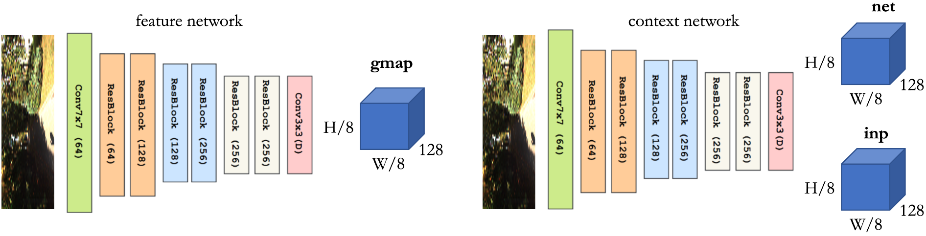 Feature and Context Networks of DROID-SLAM
Feature encoder outputs features with D = 128, which uses instance normalization. Context encoder outputs features with D = 256, no normalization is used in the context encoder. Feature network is used to build the set of correlation volumes. Context features are injected into network during application of update operator.
Correlation Pyramid
For each edge in the frame graph, $(i, j) ∈ E$, we compute a $4D$ correlation volume by taking the dot product between all-pairs of feature vectors in $g_θ(I_i)$ and $g_θ(I_j)$. Then we perform average pooling of the last two dimension of the correlation volume following to form a 4-level correlation pyramid.
 $[C^1,C^2,C^3,C^4]$ Correlation Pyramid between $I_i$ and $I_j$
Update Operator
The core component of SLAM system is a learned update operator. The update operator is a 3 × 3 convolutional GRU with hidden state $h$. Each application of the operator updates the hidden state, and additionally produces a pose update, $∆ξ (k)$ , and depth update, $∆d (k)$.
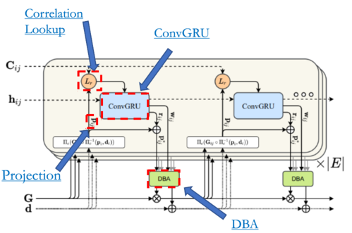
click the image hyperlinks to learn more about each module
The pose and depth updates are applied to the current depth and pose estimates through retraction on the $SE(3)$ manifold and vector addition respectively. Iterative applications of the update operator produce a sequence of poses and depths, with the expectation of converging to a fixed point ${G^k} → G^∗$ , ${d^k} → d^∗$ , reflecting the true reconstruction.
Correspondence Field $p_{ij}$
At the start of each iteration, we use the current estimates of poses and depths to estimate correspondence. Given a grid of pixel coordinates, $p_i ∈ R^{H×W×2}$ in frame $I_i$, we compute the dense correspondence field $p_{ij} ∈ R^{H×W×2} $ for each edge $(i, j) ∈ E$ in the frame graph. $p_{ij}$ represents the coordinates of pixels $p_i$ mapped into frame $I_j$ using the estimated pose and depth. $p_{ij} – p_j$ is the optical flow induced by camera motion.
 Dense Corresspondence field
${\pi}_c^{-1}$ is the inverse projection function mapping inverse depth map $d$. ${\pi}_c$ is the camera model mapping a set of $3D$ points onto the image. $fx, fy, cx, cy$ are the calibrated camera parameters. \(p_{ij}\) is used to perform lookup from the correlation volume \(C_{ij}\) to retrieve correlation features.
Correlation Lookup $L_{r}$
Lookup operator $L_{r}$ which generates a feature map by indexing from the correlation pyramid \(C_{ij}\). Given a current estimate of optical flow $(f^1 ,f^2)$, we map each pixel $I_1$ to its estimated correspondence in $I_2$. Define a local grid as set of integer offsets which are within a radius of $r$ units of $x$’ using $L_{1}$ distance. Local neighborhood $N(x’)_r$ around $x$’ is used to index the correlation volume. Lookups on all levels of the pyramid are performed, such that the correlation volume at level $k$, $C_k$ , is indexed using the grid $N(x’/{2^k})_r$.
 Lookup Operator
ConvGRU3
The GRU produces an updated hidden state $h_{k+1}$. We map the hidden state through two additional convolution layers to produce two outputs a revision flow field $r_{ij} ∈ R^{H×W×2}$ and associated confidence map $w_{ij} ∈ R^{H×W×2}$. The revision $r_{ij}$ is a correction term predicted by the network to correct errors in the dense correspondence field.
 CONV GRU Layer
Dense Bundle Adjustment Layer (DBA)
The Dense Bundle Adjustment Layer maps the set of flow revisions into a set of pose and pixelwise depth updates. \(\| . \|\) is the Mahalanobis distance which weights the error terms based on the confidence weights $w_{ij}$. Updated pose $G$’ and depth $d$’ such that reprojected points match the revised correspondence ${p^*_{ij}}$ as predicted by the update operator. We use local parameterization to linearize cost function and use the Gauss-Newton algorithm solve for updates. The system can be solved efficiently using the Schur complement with the pixelwise damping factor $λ$ added to the depth block.
 DBA Layer
Training
SLAM system is implemented in PyTorch and uses the LieTorch extension to perform backprogation. We supervise the network using a combination of pose loss and flow loss. System trained on trained on synthetic TartanAir Dataset with monocular input for 250k steps with a batch size of 4, resolution 384 × 512, and 7 frame clips, and unroll 15 update iterations. Training takes 1 week on 4 RTX-3090 GPUs.
 Loss
Loss
Inference
The SLAM system takes a video stream as input, and performs reconstruction and localization in real-time. It contains two threads which run asynchronously. The frontend thread takes in new frames, extracts features, selects keyframes, and performs local bundle adjustment. The backend thread simultaneously performs global bundle adjustment over the entire history of keyframes. In order to recover the poses of non-keyframes, we perform motion-only bundle adjustment by iteratively estimating flow between each keyframe and its neighboring non-keyframes. SLAM system can run in real-time with 2 3090 GPUs. Tracking and local BA is run on the first GPU, while global BA and loop closure is run on the second. Requires a GPU with min 24GB Memory for running in a single GPU.
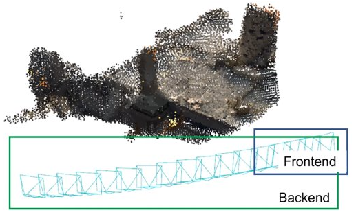 Frondend and Backend of DROID-SLAM
Evaluation
We evaluate the accuracy of the SLAM system from camera trajectory, primarily using Absolute Trajectory Error (ATE). Evaluating dense 3D reconstruction is typically considered in the domain of Multiview Stereo, which is not consider here. ATE is calcuated by first aligning the estimated trajectory to groundtruth. Then calculate the RMSE using the aligned estimation and the groundtruth trajectory.
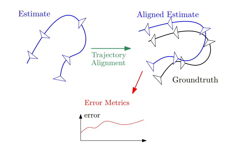 Evaluation of Camera Trajectory
Results
While prior deep learning methods are more robust, they obtain low accuracy on most of the evaluated sequences in TUM dataset, whereas classical SLAM algorithms such as ORB-SLAM tend to fail on most of the sequences. DROID-SLAM successfully tracked all 9 sequences while achieving 83% lower ATE than DeepFactors and which succeeds on all videos and 90% lower ATE than DeepV2D in TUM-RGBD dataset. We find that recent deep learning approaches perform poorly on the EuRoC dataset compared to classical SLAM systems. This is due to poor generalization and dataset biases which lead to large amounts of drif, DROID-SLAM does not suffer from these issues. DROID-SLAM is both robust and accurate.
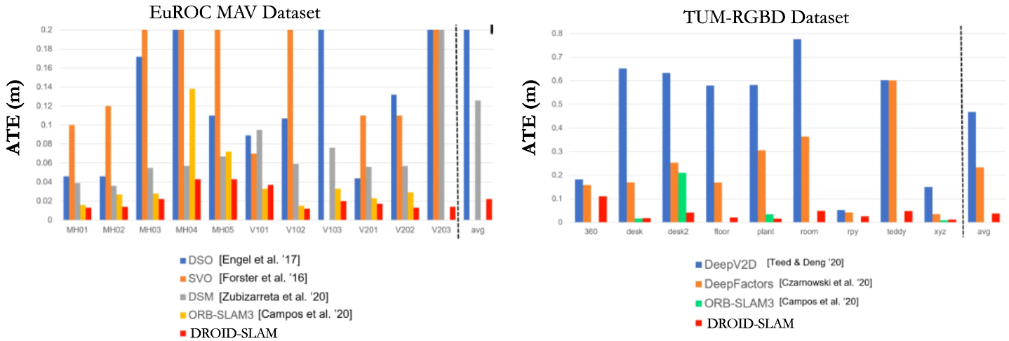 ATE : Absolute Trajectory Error (m) evaluation on realworld datasets
Monocular 3D Reconstruction
 DROID-SLAM 3D Recontruction Results
Testing on KITTI Dataset
 Testing on KITTI Dataset
These are the results you can expect from DROID-SLAM. During testing on the KITTI monocular dataset consisting of 660 images with a size of 1240 x 368, I achieved an average frame rate of 3.6 FPS, with processing taking around 3 minutes to complete.
Conclusions
DROID-SLAM, an end-to-end neural architecture for visual SLAM which is accurate, robust, and versatile and can be used on monocular, stereo, and RGB-D video.
Future Research
- Developing intuitive understanding of the mathematical concepts behind the Dense Bundle Adjustment Layer.
- Resolving the scaling problem of DORID-SLAM when working with stereo cameras.
- Exploring the potential of performing SLAM with an uncalibrated camera and obtaining calibration parameters from the DBA layer.
- Implementing multi-GPU inference to enable real-time SLAM.
- Investigating alternative representations to CONVGRU and the possibility of incorporating transformers.
- Exploring the potential of multi-camera view inference.
- Utilizing optical flow to address dynamic object removal in SLAM.
- Improving the loop closer inference mechanism.
- Developing SLAM algorithms for non-rigid objects, such as deformable or articulated structures.